Integration of Optical Systems

These application notes are relevant to both off-the-shelf and custom integration for imaging, as well as non-imaging systems. Please feel free to discuss any of the content in these notes or any other integration questions with our Applications Engineers.

Defining the Application

The first step to solving any optical problem is to assess the application. What am I trying to accomplish? For an optical system it is important to first determine whether you need an imaging system or non-imaging system because the performance requirements are different for each type.

Imaging System

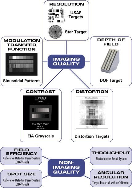
Imaging systems transfer a representation of the object to a detector, such as a camera or your eye. Some examples of imaging systems are: electronic imaging for inspection, image projection systems and relay systems. The goal of an imaging system is to provide sufficient image quality to enable extraction of desired information about the object from the image. Note that what may be adequate image quality for one application may prove inadequate in another. Some of the components of imaging quality are resolution, image contrast, perspective errors, geometric errors (such as distortion) and depth of field.

Non-Imaging System

Non-imaging systems collect, disperse, resize, focus, or collimate light. Some examples of non-imaging systems are: illumination projection, fiber coupling and laser projection. The performance of a non-imaging system can be quantified by its throughput, field efficiency, spot size (focusing systems) and angular resolution. Throughput is a measure of the energy transmitted through the lens system. Field efficiency is the system's ability to accommodate a large detector area or source size. Angular resolution is generally used to specify the minimum angular separation needed between two objects in order for the lens system to resolve them. Spot size is used to evaluate a focusing lens's performance.

The next step is to determine the primary parameters of your system. Then, you can begin a design form for your application. Below are the primary parameters defined.

Conjugate Distances

The distance from the lens to the object/source (object distance) and the distance from the lens to the detector/image (image distance). For example, in an infinite conjugate design, one of these distances approaches infinity.

Conjugate Sizes

The size of the object/source (object size) and the size of the detector/image plane (image size). For example, in systems with an infinite conjugate, the conjugate "size" can be expressed as an angle.

Numerical Aperture (NA) and f-Number (f/#)

A measure of the cone of light accepted or emitted by the lens system.

Resolution and Spot Size

In imaging system terms, this refers to the smallest feature of an object distinguishable by the system. (This value may be magnification limited or diffraction-limited). In non-imaging systems, spot size is a way to characterize the performance needed. Infinite conjugate systems are often defined in terms of angular resolution.

Solution Forms

Most application solutions can be divided into three types of designs: Finite/Finite Conjugate, Infinite/Infinite Conjugate, or Infinite/Finite Conjugate. A finite/finite conjugate design is one in which light from a source (not at infinity) is focused down to a spot. Most video lenses, which take the image of an object at a finite distance away and focus it onto a sensor, are designed for this scenario. An infinite/infinite conjugate application takes incoming collimated (parallel) light, changes the beam diameter according to the magnification, and emits the collimated light. An infinite/finite conjugate design combines these two concepts by focusing a source placed at infinity down to a small spot.

In order to choose the appropriate design, it is best to begin with the "paraxial solution." A paraxial solution allows a designer to approximate first-order properties such as conjugate distances, image and object heights, magnification, etc. Paraxial calculations utilize paraxial elements - theoretically perfect lenses that do not introduce system aberrations associated with lens thickness, radius of curvature, glass type and dispersion effects. Note: the only specifications for a paraxial lens are its position relative to the image and object plane, lens diameter, and focal length. After finding the paraxial solution you can begin to select the best real lens solution for your application, making allowances for lens thickness, dispersion effects, etc. in your calculations. Because the calculations for real lens solutions can be long and tedious, optical design software helps system designers integrate optics into their applications and see how they will perform. Common optical design software packages include OpticStudio from Zemax and CODE V from Synopsis.

Each design form below illustrates different lens combinations and the performance associated with them. Please note that you are not limited to just these lens combinations. Below is a list of variables used for the solution examples.

Description of Variables;
$$ H_i, \,  H_o $$	Image and object height, respectively. This represents HALF of the actual full image and object size. In afocal systems, this represents half of the full beam waist.
$$ I, \, O $$	Image and object distance measured from the lens closest to the image and object respectively.
$$ F_i, \,  F_o $$	Focal length of the lens closest to the image and object, respectively.
$$ F $$	Effective focal length of the entire lens system.
$$ M $$	Magnification is the system's ability to produce an enlarged/reduced image or projection of an object.
$$ d $$	Distance between two elements.
$$ \theta $$	FULL angle of the cone of light accepted or emitted by a lens system (closely linked to numerical aperture).
$$ \alpha_i, \, \alpha_o $$	Angular HALF field of view in infinite conjugate systems.
$$ \text{TP} $$	Throughput is the system's ability to transfer light.
$$ f / \# $$	f/# is the lens' ability to focus light.
$$ D $$	Diameter of the Lens

Sign Convention

Positive Values: The following quantities are expressed as positive values: heights above the optical axis, distances measured to the right of a reference point, focal length of focusing lenses, and angles that are measured counterclockwise from the optical axis.

Negative Value: The opposites of the above quantities are expressed as negative values. (i.e. - While height measured above the optical axis is expressed as a positive quantity, height measured below the optical axis is expressed as a negative quantity).

Reference Point for Equations Given: Lens Position

CASE 1: FINITE/FINITE CONJUGATES

Common Applications: Electronic Imaging, Relay Systems and Image Projection

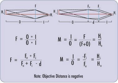
Single Element: The simplest form of a finite/finite conjugate system is one with a single element in which the effective focal length of the system is equal to the focal length of the single lens. Some advantages of this design are its cost effectiveness and its simplicity of design. The following equations determine the first order optical properties of a single lens.

Two Element: You can combine elements to achieve different effective focal lengths while increasing the image performance of the system drastically. The design becomes a bit more complex, though one method of simplifying it is to place the object at the focal point of the object lens and the image at the focal point of the image lens.

Real Lens Solutions: For imaging applications, achromats are typically used in order to yield better image quality with a single element. Singlets (PCX or DCX) are typically used in illumination based relays which do not require high resolution.

Single Element | Two Element

Lens Type	Low f/#	Polychromatic	Field Efficiency	Cost	Suggested Applications
Plano-Convex (PCX)	•	•	••	$\small{ \$ \$ } $	use in pairs
Double-Convex (DCX)	••	•	•••	$ \small{ \$ } $	single element
Achromat	••••	••••	••••	$ \small{ \$ \$ \$ \$ } $	use in pairs
Hastings	••••	•••••	••••	$ \small{ \$ \$ \$ \$ \$ } $	use in pairs
Steinheil	•••••	•••••	•••••	$ \small{ \$ \$ \$ } $	single element

CASE 2: INFINITE/INFINITE CONJUGATES

Common Applications: Telescopes and Laser Beam Expanders

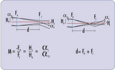
One Positive Element and One Negative Element: Most high-power laser applications utilize this form for beam expansion. One advantage of this form is that system length is greatly reduced while an erect image is maintained.

Two Positive Elements: Using two positive elements yields an intermediate image which is useful for applications requiring use of a crosshair or other type of reticle. Using two positive elements will result in a negative magnification such that a prism erector or intermediate relay lens would be needed for erect image viewing.

Real Lens Solutions: Achromatic lenses are typically used for improving field efficiency.

Note: Eyepiece designs can be used as the imaging lens to improve performance.

One Positive, One Negative Two Positive

Lens Type	Low f/#	Polychromatic	Field Efficiency	Cost	Suggested Applications
Plano-Convex (PCX)	••	•	••	$ \small{ \$ \$ } $	imaging, illumination
Double-Convex (DCX)	•	•	••	$ \small{ \$ \$ } $	-
Achromat	••••	••••	••••	$ \small{ \$ \$ \$ \$ } $	imaging, illumination
Hastings	••••	•••••	•••••	$ \small{ \$ \$ \$ \$ \$ } $	imaging, illumination
Steinheil	•••	•••••	••	$ \small{ \$ \$ \$ \$ \$ } $	-

CASE 3: INFINITE/FINITE CONJUGATES

Common Applications: Autocollimators, Light Detection, and Infinity Corrected Objectives

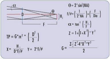
Single Element: Except in the case of infinity-corrected objectives, this solution generally does not require the use of more than one element, and the image can be found at the focal point of the lens. An important function of an infinite/finite conjugate system is the throughput (flux per unit radiance or luminance) seen by the detector. The following paraxial equations can be used to estimate the amount of throughput generated by the lens system.

Real Lens Solutions: A singlet will provide sufficient results for most applications that focus an extended light source upon a detector.

Lens Type	Low f/#	Polychromatic	Field Efficiency	Cost	Suggested Applications
Plano-Convex (PCX)	••	•	••	$ \small{ \$ } $	detector, illumination
Double-Convex (DCX)	•	•	••	$ \small{ \$} $	—
Achromat	••••	••••	••••	$ \small{ \$ \$ } $	imaging
Hastings	•••••	•••••	•••••	$ \small{ \$ \$ \$ } $	imaging
Steinheil	•••	•••••	•••	$ \small{ \$ \$ \$ } $	—

Application Example: Finite/Finite Conjugate

A typical Finite/Finite Conjugate application is wire bond inspection. First, we will define the necessary parameters. Field of view (object size) required is 5mm. The imaging sensor is a ½" format CCD with a horizontal sensing distance of 6.4mm. Unfortunately, due to the size of the probes, the object distance must be 50mm or greater. Neither the image nor the object distance is at infinity, so the Finite/Finite Conjugate design form can be used to solve this example.

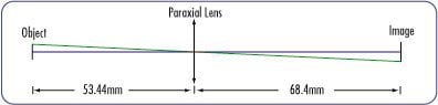
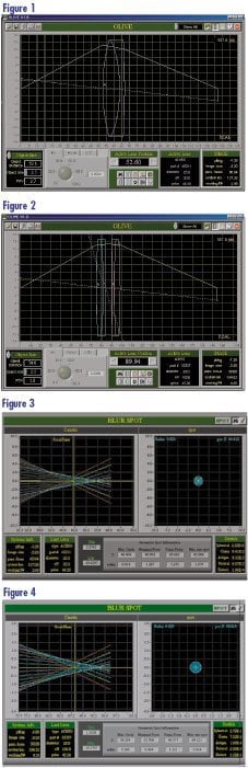
The next step is to find a real lens that solves your application requirements. Based on our solution above we need a lens with a focal length of 28.07mm. Since this is an imaging application, achromats can be used to improve image quality. A good lens choice would be to use a 25mm diameter achromat with 30mm focal length (#45-211 Achromatic Doublet), given that a focal length of 28.07mm is not available off-the-shelf. Inserting this lens into lens design software, we can easily find the actual object and image distance (i.e. the real lens solution) that we must position the lens at. Below is a diagram of the paraxial lens solution. The chart below summarizes the differences between the paraxial and real lens solutions. The paraxial equations steered us in the right direction and helped narrow down the lens choices while inserting the real lens gave precise answers for the image and object distance.

Parameter	Paraxial Solution	Real Lens Solution	Real Lens Solution
Lens System	Single Achromat	Single Achromat	Achromat Pair
Effective Focal Length	30mm	30mm	75 / 100mm
Magnification	1.28X	1.28X	1.28X
Object Distance	53.44mm	56.2mm	74.81mm
Paraxial Image Distance	68.4mm	60.460mm	96.08mm
Best Focus Location	unknown	44.404mm	88.28mm

Due to aberrations associated with real lenses, design software gives a minimum spot size of 0.9mm (see Figure 3) for the single 25mm Dia x 30mm FL achromat in the given configuration. Inserting an achromat pair (#55-280) reduces this spot size to 0.3mm which equates to an increase in resolution (reference Figures 2 and 4). An aperture can be inserted between the two achromats for a further increase in performance. This is a prime example of how paraxial knowledge along with software such as OpticStudio or CODE V can help to improve your imaging solutions.

Mechanical Integration

Once optical layout is defined it needs to be integrated into a mechanical housing. In doing so, lens spacing must be maintained despite the effects of sag. Once sag for each surface is determined, spacers and seats can be designed to yield appropriate center-to-center lens spacing.

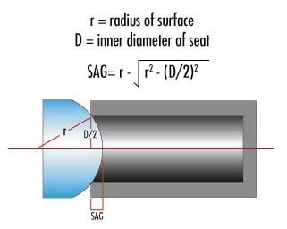
Sag

Sag is the distance between the edge of a mount and the vertex of a surface (see illustration below). Sag only exists when surfaces have curvature, as the inner diameter of the spacer or seat determines vertex location.

Retainer vs. Spacer

The three common lens-mounting techniques are: retainer rings, spacers and a combination thereof. Retainers generally offer tighter control over the elements' position, tilt and centering because the lens sits on a counterbored seat. Retainers can be costly and are sometimes impractical in small assemblies. Spacers are ideal for small assemblies and are cost-effective though they yield looser lens spacing tolerance than with retainer rings.

Focusing/Adjustment

All optical designs require some focusing or adjustment. Common focusing techniques are moving the image (sensor), object or lens elements.

Tolerances

Tolerances affect the yield of a production lens. Because each dimension has an associated tolerance, yield is less than 100%. The conventional method of stacking up tolerances tends to result in over-toleranced (and overpriced) designs. Instead, by combining each probability curve, one can accurately predict the % yield of a lens. Understanding the probabilistic nature of tolerancing is vital to reducing the per piece cost in large production runs.

TESTING AND EVALUATION

Once a system is assembled, its parameters must be quantified to determine whether the application requirements have been met. During prototyping, slight alterations to the original design are typical to accommodate component limitations.

Fundamental Parameters

Every application has first-order requirements (e.g. conjugate distances, magnification). Paraxial calculations, which do not take into account the properties of the glass(dispersion, thickness, etc.), may need adjustment to meet first-order requirements.

Design Performance

Since paraxial calculations do not indicate real-world performance, image quality of the assembly should be tested. Various targets exist for determining the quality of imaging systems. Non-imaging systems may require more involved interferometric instruments for testing.

Resolution and Contrast: can be measured using the USAF and EIA Grayscale targets respectively. Perspective errors can be determined by measuring magnification change across the depth of field.

Throughput: can be measured as power with a photodiode. A CCD analyzes spot size and beam profiling. Collimator measures angular resolution.

RULES OF THUMB:

Test with Application in Mind: Do not test performance beyond what the application requires. Test only critical parameters to reduce costs.

Cost Associated with Testing: Testing adds significant costs. High-volume production warrants extra testing resources though low-quantity production does not justify it.

Visual Tests:

Tests based on a visual observation are subjective and lack repeatability. Because the human eye can extrapolate missing information, visual tests need to be desensitized to human error (e.g. utilize a line profile function across the USAF resolution target to determine the actual Group and Element that are resolvable.)